Creative and daring ways
Anisotropic visco-elastic FWI of an offset VSP dataset
This case study has been presented in the 2010 annual meeting of the SEG.
This dataset is from North Sea. The case is a particular well seismic with only 2 sources with offset at the surface (marine well seismic).
This dataset is from North Sea. The case is a particular well seismic with only 2 sources with offset at the surface (marine well seismic).
The Lille Friegg context and the poor quality of migrated images
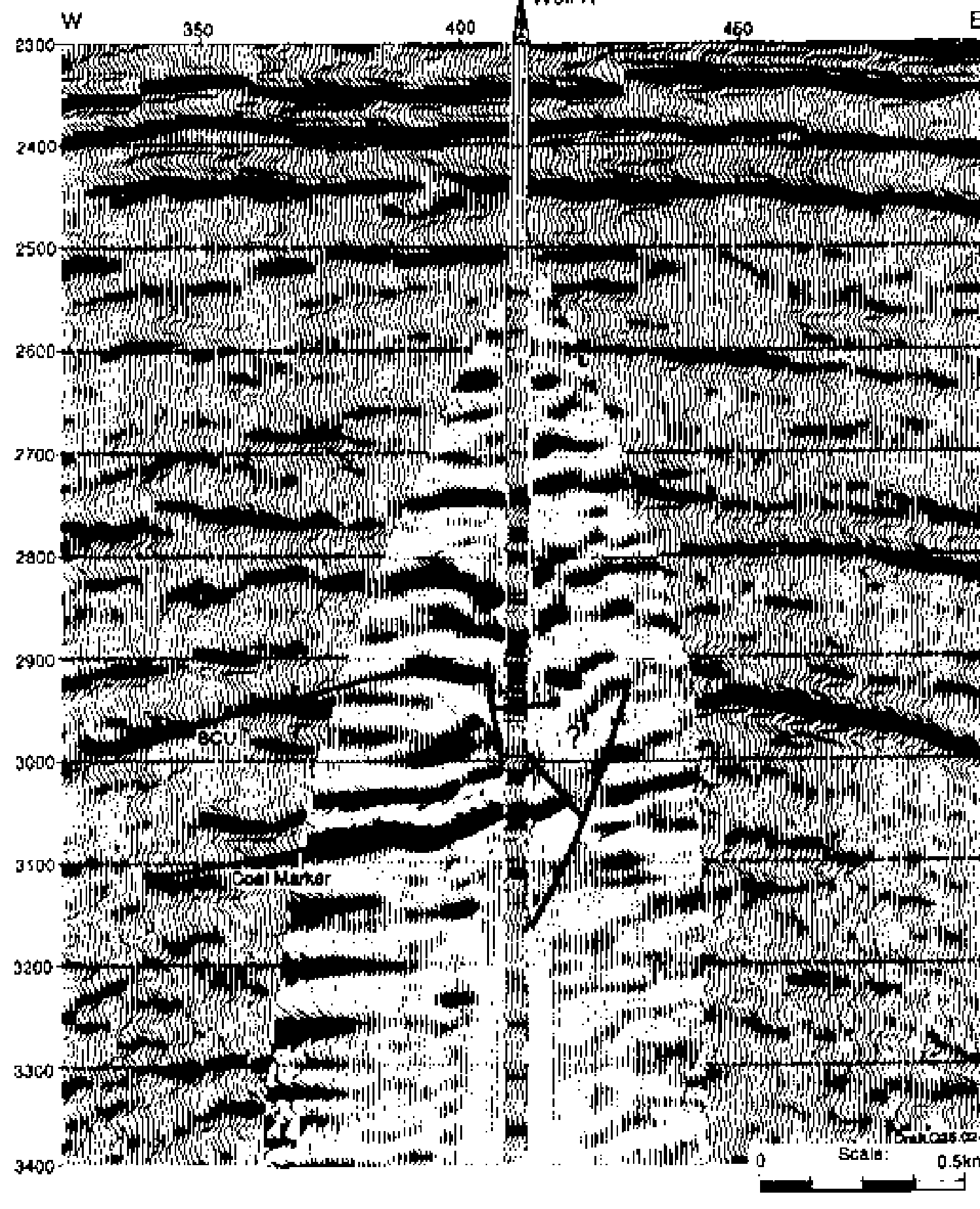
The location of the field is west of Norway and surface seismic migrated images were very poor (see images below). Seismic data were acquired in the early 90ties but the quality is quite good.
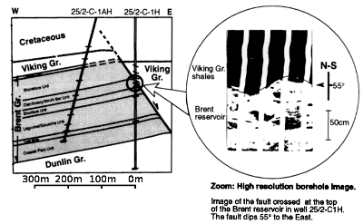
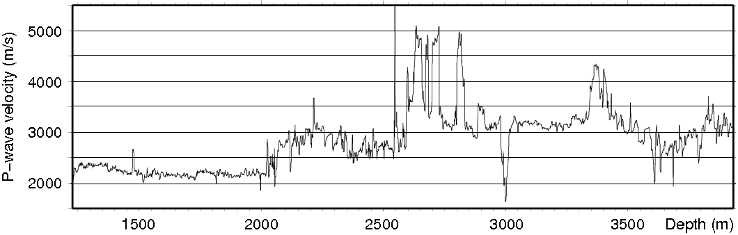
The history is that the first well, vertical, did not cross the upper part of the brent formation (in gray) where the gas was trapped, it crossed only the lower part of the formation ... dry. Decision was taken to acquire well seismic (see the migrated offset VSP images in the surface migrated image below) but the resolution could not be improved due to massive limestone bars around 2700m depth with high reflectivity above the target reservoir (see the sonic logs below) and for some other reasons. The geological interpretation is from Minsaas, Kravik and Haller (1994)1.
The location of the field is west of Norway and surface seismic migrated images were very poor (see images below). Seismic data were acquired in the early 90ties but the quality is quite good.
The history is that the first well, vertical, did not cross the upper part of the brent formation (in gray) where the gas was trapped, it crossed only the lower part of the formation ... dry. Decision was taken to acquire well seismic (see the migrated offset VSP images in the surface migrated image below) but the resolution could not be improved due to massive limestone bars around 2700m depth with high reflectivity above the target reservoir (see the sonic logs below) and for some other reasons. The geological interpretation is from Minsaas, Kravik and Haller (1994)1.
The question was: Can waveform inversion help us better define the structure,
delineate and characterize the gas bearing brent reservoir?
delineate and characterize the gas bearing brent reservoir?
The global strategy to overcome the problems
Extract more information from the data while decreasing the number of degrees of freedom
On the data space, we had small amount of data, weak redundancy but a complex and informative wavefield. Decisions were: not separate or remove part of the data, use adequate rheology in order to well reproduce the data and decrease the modeling noise (at least elastic for low frequency and viscolastic for high frequency inversion), and invert 1st , 2nd and 3rd order scattered waves: multiples or conversions.
On the model space, we had 2D structures which involve 2D inversion and in order to obtain the good amplitudes (geometrical spreading and amplitude of inverted multiples), we performed a 2.5D modeling. We used both horizontal and vertical correlations in order to decrease the number of degrees of freedom in the inverse problem and we worked to find a good starting model for the different parameter fields.
The results for the final estimated model of the FWI
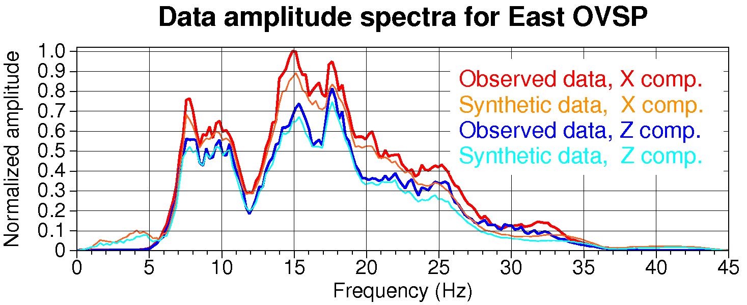
The results are shown both in the data space and in the model space.
The results are shown both in the data space and in the model space.
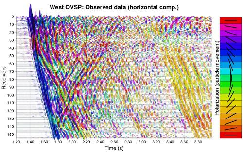
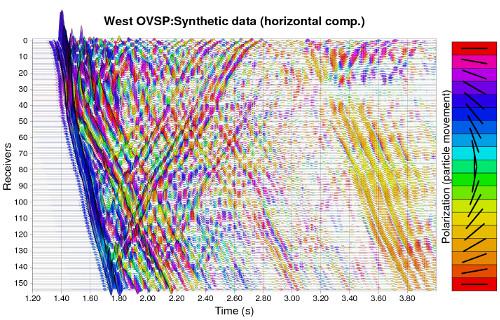
As shown on the seismograms just above, all the data phases are retrieved, first order as the direct P-wave (first arrival), second order as the water bottom multiple, converted P to S waves or reflection P-S on the reservoir top and bottom (upgoing wave from the receiver 140), the S wave from the first layer under the water bottom (yellow phases at right) and third order phases as P-S-P converted from the latter phase to P wave reflected on the top of the limestone bars.
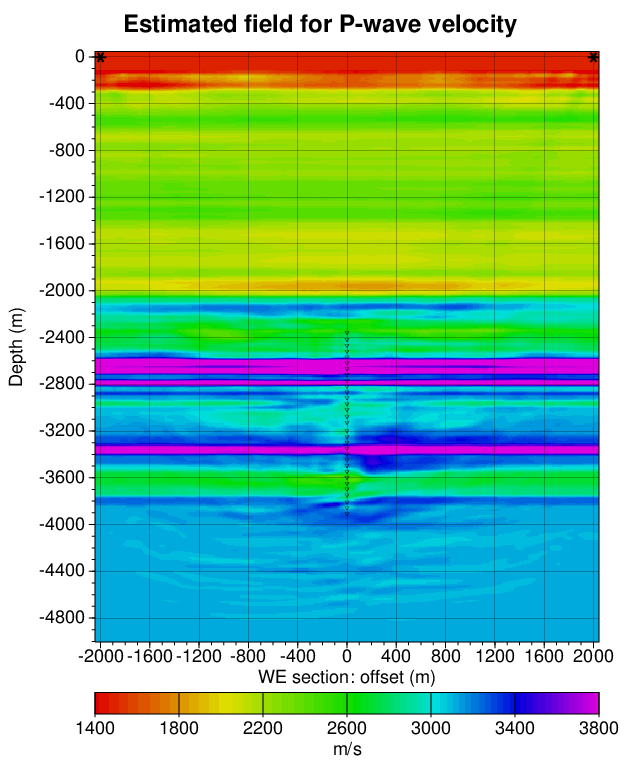
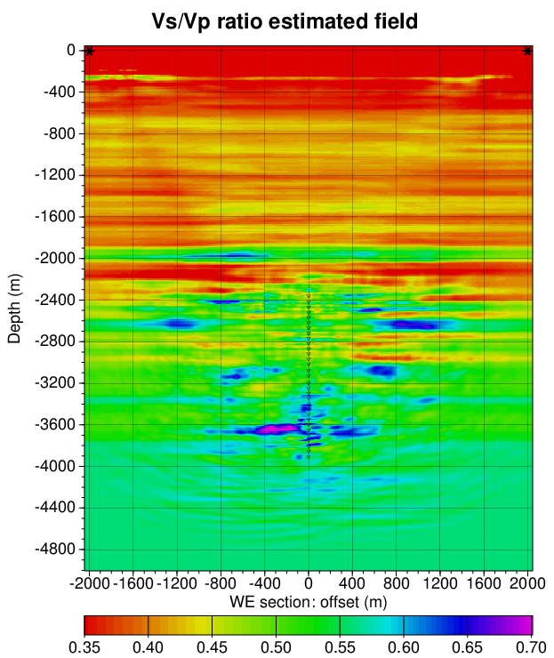
The two plots above are the P-wave velocity estimated field at left and the Vs/Vp ratio estimated field at right. The stars at the surface denote the location of the sources for both shots, west and east OVSP. The triangles in the center of the images (0m offset), from 2400m down to 3700m depth represent the antenna of receivers. The resolution is good in the antenna vicinity and we see at the reservoir depth (3600m) the gas in the reservoir only on the left side of the well. Zooms are provided below.

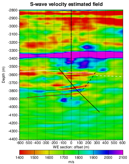
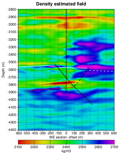
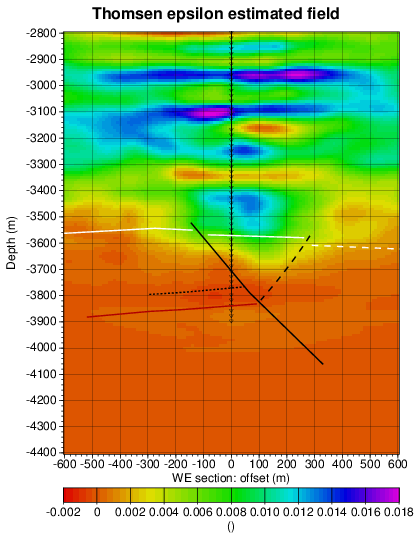
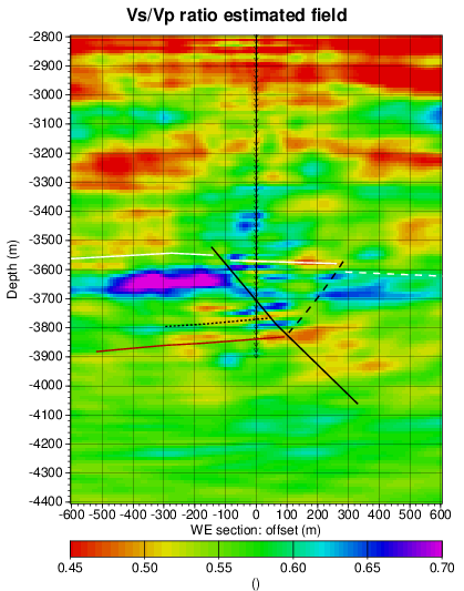
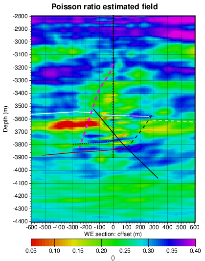
Details of the final estimated field (fourth step of the Full-Wave Inversion with f0 = 20Hz) with the geological interpretation given in Minsaas, Kravik and Haller (1994). The solid black line indicates the fault while the dashed black line denotes a likely secondary fault. The white line is the unconformity at the top of the Brent formation. The dotted black line denotes a coal thin layer, good seismic marker, and the dark red solid line the bottom of the Brent formation. The well antenna is indicated by small triangles and the deviated well (side-track) by the pink dashed thick line on the last diagram. The P-wave estimated velocity field (top left) is not very discriminative and spatial resolution is poor, the S-wave estimated velocity field (top center) has much better spatial resolution and exhibits some interesting detail while the density estimated field (top right) provides some additional information for reflectivity like the coal layer in red. The Thomsen epsilon estimated field (bottom left) is not significant showing that the 2 sources are not sufficient to obtain a good resolution on anisotropic parameters. Both the two last diagrams, Vs/Vp ratio estimated field (bottom center) and Poisson ratio estimated field (bottom right), show the same structures: the gas bearing upper part of the Brent reservoir respectively in pink and in red. The low values of the Poisson ratio indicate typically the presence of gas.
Conclusions
These results obtained thanks to the accurate seismic modeling and the Full-Wave Inversion technique has been checked by geophysicists: depths of structures are correctly retrieved and low values of Poisson ratio are a little underestimated. The overall results are excellent compared to results obtained using standard techniques as migration from surface or for well seismic data.
These results obtained thanks to the accurate seismic modeling and the Full-Wave Inversion technique has been checked by geophysicists: depths of structures are correctly retrieved and low values of Poisson ratio are a little underestimated. The overall results are excellent compared to results obtained using standard techniques as migration from surface or for well seismic data.
1 O. Minsaas, K. Kravik & D. Haller. Integration of exploration and reservoir approaches through geophysical and geological technologies in mature area. In Proceedings of the 14th World Petroleum Congress, 77, 1994.